In the previous blog post, while fitting the transfer function equation to the measurement data, I emphasized on the importance of having realistic and sensible Starting Values for the fitting algorithm to achieve good fit while also estimating sensible values of parameters. This is always easier said than done. I have always felt that, one has to think in so many different ways than one to make the algorithm run such that the outcomes it generates make sense.
One of the techniques that I use to arrive at reasonable starting point values, apart from actual measurements of individual parameters (wherever possible), is to understand what each parameter in the transfer function does, or affects the response of the transfer function. In this case, the impedance transfer function depends on Bl, Re, Le, Mmd, Rms and Cms. In the MATLAB Curve Fitting toolbox, I start with some random guesses for at least one or two parameter values which make sense to me. Sometimes there is absolutely no fit at the end of the algorithm execution giving a flat line and I end up doing some trial and error to atleast get a peak or shape of some sort (anything other than an absolutely FLAT line). Once you get a shape that somewhat resembles the intended transfer function shape as seen on the measurement data, I adjust the Starting Point values of the parameters in a way that I can direct the current output of the algorithm to approach the shape of measured data.
To make it clearer, I generated some plots where I vary one parameter at a time and plot the transfer function (impedance) for 3 different values of the same parameter. (all this, while keeping the other parameters constant) I have modelled the impedance here based on the parameter values estimated for the Ole Wolff driver that is being studied. I repeat this exercise for each of the 6 parameters that influence the transfer function response.
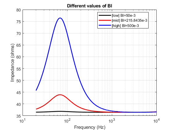
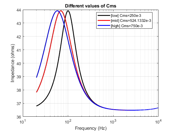
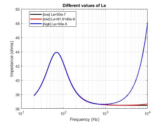
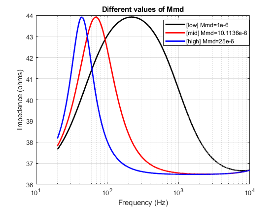
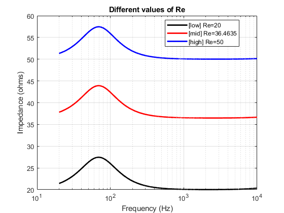
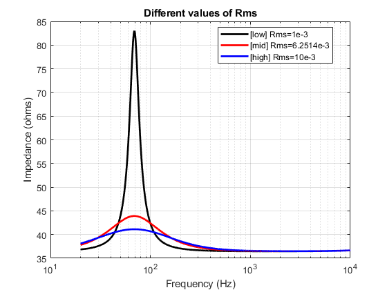
The mid value of each parameter used for plotting here are the values estimated from yesterday’s post. The low and high values are just randomly chosen values to illustrate the effect of the parameter on the transfer function so that it is easier to compare and understand.
Summary
To summarize, it can be seen that each of the parameters affects the resonance on a few different aspects like,
- Q factor of the peak
- Central Frequency of the peak
- Amplitude of the peak
- Base level position of the function (along the vertical axis)
There are also parameters which affect the transfer function on not just one aspect but a combination of multiple aspects. This information/understanding is often quite useful to decide better estimates of starting values for each of the parameters while performing trial and error. This way, you can ensure that you are not being totally random, but making judgements while being grounded in a scientific understanding of the underlying phenomenon.