Now that the complete circuit representing the lumped model for the Ole Wolff driver in consideration has been developed, we need to find the component values for each of the R, L and C components in the circuit so that it fully mimics the behavior of the actual driver and matches the measured response. However, since I already stated that the formulae for finding those component values are based purely on empirical relations, they might not lead to a system transfer function that ‘exactly’ matches that of the measured transfer function responses of the driver that’s available on the product website. Hence the parameter values are estimated by Curve Fitting to the measured data, like it was done for the case where electro-mechanical circuit component values were obtained from data of the driver when measured in vacuum. (atleast with ‘simulated’ vacuum data like I generated in one of the earlier posts) To do this, the circuit transfer function equations are required. It was done before for the purely electro-mechanical circuit without the acoustical circuit included. However, since the acoustic circuit is now available and corresponding changes were also made to the mechanical circuit, a new set of equations are to be derived. So, I will start with deriving the circuit equations now, in this post, and then go on to calculating the empirical values of components in the subsequent posts.
The circuit equations are derived by applying Kirchoff’s Current and Voltage laws. Before identifying nodes and loops/current meshes in the circuit, it’s worthwhile noting if there are areas which could be clubbed together/reduced into one element for simplifying the circuit and making the circuit equations simpler to look at.

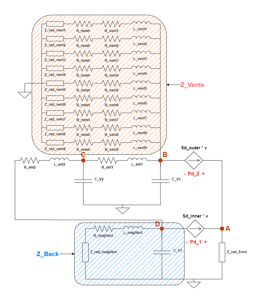
As can be seen above, there are 4 nodes that have been identified in the circuit where we could define the current and voltage equations for circuit analysis and some components have been clubbed together in a way that they could be modelled as one impedance component for simplification. The part of the circuit marked by the RED hatched area, comprises of the circuit elements related to the vents in the back of the driver’s plastic enclosure. Here we can see that each branch is the same type and 9 such branches are connected in parallel. So the impedances of components in series can be added together and 9 such branches can be added in parallel; hence the clubbing of this part of the circuit into an effective impedance value called Z_Vents. The BLUE hatched region is also suitable for simplification since we can see 2 branches connected at node D on one side and grounded on the other, once again forming a parallel connection. This part of the circuit can be modelled by an effective equivalent impedance called Z_Back. The mathematical expressions of these impedances would be shared further down in this article.

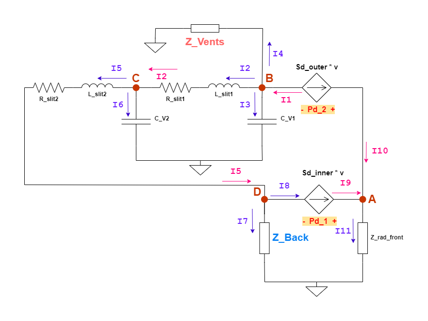
The circuit has been simplified by replacing the circuit blocks marked before with the corresponding equivalent impedances and the nodes (A, B, C, D) have been marked. The currents entering and exiting the nodes have been marked. The currents entering any given node is marked PINK in color and the currents exiting the node are marked PURPLE in color, for ease of identification. The direction pointed to by the arrow heads of the 2 current sources are considered as the Positive direction as a convention here.
The equations for each of the nodal currents and nodal voltages at the identified nodes can be laid out as below.
Note: The terms of the form $X_{Cxx}$ are capacitive reactances and $X_{Lxx}$ are inductive reactances whose values are calculated as follows
$X_{Cxx}\ =\frac{1}{\omega\cdot\ Cxx}$
$X_{Lxx} = \omega \cdot Lxx$
Looking at the current and voltage components around node A ($V_A$ is the potential/voltage at node A)
| $I11 = I9 + I10$ | (1) |
| $I9 = v \cdot Sd\_inner$ | (2) |
| $I10 = v \cdot Sd\_outer$ | (3) |
| $\begin{align} V_A &= I11 \cdot Z\_rad\_front \\ &= \left ( v \cdot Sd\_inner + v \cdot Sd\_outer \right ) \cdot Z\_rad\_front \\ &= v \cdot \left (Sd\_inner + Sd\_outer \right) \cdot Z\_rad\_front \end{align}$ | (4) |
At node B
| $I1 = -v \cdot Sd\_outer$ | (5) |
| $I1 = I2 + I3 +I4 $ | (6) |
| $I3 = \frac{V_B}{X_{C\_V1}}$ | (7) |
| $I4 = \frac{V_B}{Z\_Vents}$ | (8) |
At node C
| $I2 = I5 + I6$ | (9) |
| $I6 = \frac{V_C}{X_{C\_V2}}$ | (10) |
The current $I2$ can be expressed also as
| $I2 = \frac{V_B\ -\ V_C}{R\_slit1\ +\ X_{L\_slit1}}$ | (11) |
The current $I5$ can be expressed also as
| $I5 = \frac{V_C\ -\ V_D}{R\_slit2\ +\ X_{L\_slit2}}$ | (12) |
Substituting (11), (12) and (10) in (9)
| $\frac{V_B\ -\ V_C}{R\_slit1\ +\ X_{L\_slit1}} = \frac{V_C\ -\ V_D}{R\_slit2\ +\ X_{L\_slit2}} + \frac{V_C}{X_{C\_V2}}$ |
On re-arranging the terms, we have,
| $V_C = \frac{\frac{V_B}{R\_slit1+X_{L\_slit1}} + \frac{V_D}{R\_slit2+X_{L\_slit2}} }{ \frac{1}{R\_slit1+X_{L\_slit1}} + \frac{1}{R\_slit2+X_{L\_slit2}} + \frac{1}{X_{C\_V2}} }$ |
| (13) |
At node D
| $I5 = I7 + I8$ | (14) |
| $I7 = \frac{V_D}{Z\_Back}$ | (15) |
| $I8 = v \cdot Sd\_inner$ | (16) |
Substituting (12), (15) and (16) in (14)
| $\frac{V_C\ -\ V_D}{R\_slit2\ +\ X_{L\_slit2}} = \frac{V_D}{Z\_Back} + v \cdot Sd\_inner$ |
Upon re-arranging terms we have,
| $V_D = \frac{Z\_Back \cdot \left [ V_C\ -\ (v) \cdot (Sd\_inner) \cdot \left (R\_slit2\ +\ X_{L\_slit2} \right ) \right ] }{R\_slit2\ +\ X_{L\_slit2}\ +\ Z\_Back}$ |
| (17) |
Substituting (5), (11), (7) and (8) in (6)
| $-v \cdot Sd\_outer\ =\ \frac{V_B\ -\ V_C}{R\_slit1\ +\ X_{L\_slit1}}\ +\ \frac{V_B}{X_{C\_V1}}\ +\ \frac{V_B}{Z\_Vents}$ |
Upon re-arranging terms we have,
| $V_B\ =\ \frac{1}{ \left ( \frac{1}{R\_slit1+X_{L\_slit1}}\ +\ \frac{1}{X_{C\_V1}}\ +\ \frac{1}{Z\_Vents} \right ) } \left [\frac{V_C}{R\_slit1+X_{L\_slit1}}\ -v \cdot Sd\_outer \right ]$ |
| (18) |
There are 3 linear equations with 3 unknowns $V_B$, $V_C$ and $V_D$ now which have to be solved to obtain the expression for each term which is independent of the other two. I’m too lazy to solve this. 😛 So I sought help of Maple to solve these equations for me. And I have 3 super long expressions for each of the 3 potentials. Sharing them here for your reference.
${V_B} {=} -\frac{\textcolor{red}{\textbf{v}} \cdot \textit{Z_}\mathit{Vents} \cdot \left(\left(\textit{X_}\mathit{Lslit1} \textit{Sd_}\mathit{outer}+\textit{Sd_}\mathit{outer} \textit{R_}\mathit{slit1}+\left(\textit{R_}\mathit{slit2}+\textit{X_}\mathit{Lslit2}+\textit{Z_}\mathit{Back}\right) \textit{Sd_}\mathit{outer}+\textit{Z_}\mathit{Back} \textit{Sd_}\mathit{inner}\right) \textit{X_}\mathit{CV2}+\textit{Sd_}\mathit{outer} \left(\textit{R_}\mathit{slit2}+\textit{X_}\mathit{Lslit2}+\textit{Z_}\mathit{Back}\right) \left(\textit{R_}\mathit{slit1}+\textit{X_}\mathit{Lslit1}\right)\right) \cdot \textit{X_}\mathit{CV1}}{\left(\left(\textit{X_}\mathit{Lslit1}+\textit{X_}\mathit{Lslit2}+\textit{X_}\mathit{CV1}+\textit{Z_}\mathit{Back}+\textit{R_}\mathit{slit1}+\textit{R_}\mathit{slit2}\right) \textit{Z_}\mathit{Vents}+\textit{X_}\mathit{CV1} \left(\textit{X_}\mathit{Lslit1}+\textit{X_}\mathit{Lslit2}+\textit{Z_}\mathit{Back}+\textit{R_}\mathit{slit1}+\textit{R_}\mathit{slit2}\right)\right) \textit{X_}\mathit{CV2}+\left(\textit{R_}\mathit{slit2}+\textit{X_}\mathit{Lslit2}+\textit{Z_}\mathit{Back}\right) \left(\left(\textit{X_}\mathit{Lslit1}+\textit{X_}\mathit{CV1}+\textit{R_}\mathit{slit1}\right) \textit{Z_}\mathit{Vents}+\textit{X_}\mathit{CV1} \left(\textit{R_}\mathit{slit1}+\textit{X_}\mathit{Lslit1}\right)\right)}$
${V_C}{=}-\frac{\textcolor{red}{\textbf{v}} \cdot \textit{X_}\mathit{CV2} \cdot \left(\left(\left(\left(\textit{Sd_}\mathit{inner}+\textit{Sd_}\mathit{outer}\right) \textit{Z_}\mathit{Back}+\textit{Sd_}\mathit{outer} \left(\textit{R_}\mathit{slit2}+\textit{X_}\mathit{Lslit2}\right)\right) \textit{X_}\mathit{CV1}+\textit{Z_}\mathit{Back} \textit{Sd_}\mathit{inner} \left(\textit{R_}\mathit{slit1}+\textit{X_}\mathit{Lslit1}\right)\right) \textit{Z_}\mathit{Vents}+\textit{X_}\mathit{CV1} \textit{Z_}\mathit{Back} \textit{Sd_}\mathit{inner} \left(\textit{R_}\mathit{slit1}+\textit{X_}\mathit{Lslit1}\right)\right) }{\left(\left(\textit{X_}\mathit{Lslit2}+\textit{X_}\mathit{CV2}+\textit{Z_}\mathit{Back}+\textit{R_}\mathit{slit2}\right) \textit{X_}\mathit{CV1}+\left(\textit{X_}\mathit{Lslit1}+\textit{X_}\mathit{CV2}+\textit{R_}\mathit{slit1}\right) \textit{Z_}\mathit{Back}+\left(\textit{X_}\mathit{Lslit1}+\textit{X_}\mathit{Lslit2}+\textit{R_}\mathit{slit1}+\textit{R_}\mathit{slit2}\right) \textit{X_}\mathit{CV2}+\left(\textit{R_}\mathit{slit1}+\textit{X_}\mathit{Lslit1}\right) \left(\textit{R_}\mathit{slit2}+\textit{X_}\mathit{Lslit2}\right)\right) \textit{Z_}\mathit{Vents}+\left(\left(\textit{X_}\mathit{Lslit1}+\textit{X_}\mathit{CV2}+\textit{R_}\mathit{slit1}\right) \textit{Z_}\mathit{Back}+\left(\textit{X_}\mathit{Lslit1}+\textit{X_}\mathit{Lslit2}+\textit{R_}\mathit{slit1}+\textit{R_}\mathit{slit2}\right) \textit{X_}\mathit{CV2}+\left(\textit{R_}\mathit{slit1}+\textit{X_}\mathit{Lslit1}\right) \left(\textit{R_}\mathit{slit2}+\textit{X_}\mathit{Lslit2}\right)\right) \textit{X_}\mathit{CV1}}$
${V_D} {=}-\frac{\textcolor{red}{\textbf{v}} \cdot \textit{Z_}\mathit{Back} \cdot \left(\left(\left(\left(\textit{Sd_}\mathit{inner}+\textit{Sd_}\mathit{outer}\right) \textit{X_}\mathit{CV2}+\textit{Sd_}\mathit{inner} \left(\textit{R_}\mathit{slit2}+\textit{X_}\mathit{Lslit2}\right)\right) \textit{X_}\mathit{CV1}+\left(\left(\textit{X_}\mathit{Lslit1}+\textit{X_}\mathit{Lslit2}+\textit{R_}\mathit{slit1}+\textit{R_}\mathit{slit2}\right) \textit{X_}\mathit{CV2}+\left(\textit{R_}\mathit{slit1}+\textit{X_}\mathit{Lslit1}\right) \left(\textit{R_}\mathit{slit2}+\textit{X_}\mathit{Lslit2}\right)\right) \textit{Sd_}\mathit{inner}\right) \textit{Z_}\mathit{Vents}+\left(\left(\textit{X_}\mathit{Lslit1}+\textit{X_}\mathit{Lslit2}+\textit{R_}\mathit{slit1}+\textit{R_}\mathit{slit2}\right) \textit{X_}\mathit{CV2}+\left(\textit{R_}\mathit{slit1}+\textit{X_}\mathit{Lslit1}\right) \left(\textit{R_}\mathit{slit2}+\textit{X_}\mathit{Lslit2}\right)\right) \textit{Sd_}\mathit{inner} \textit{X_}\mathit{CV1}\right)}{\left(\left(\textit{X_}\mathit{Lslit2}+\textit{X_}\mathit{CV2}+\textit{Z_}\mathit{Back}+\textit{R_}\mathit{slit2}\right) \textit{X_}\mathit{CV1}+\left(\textit{X_}\mathit{Lslit1}+\textit{X_}\mathit{Lslit2}+\textit{Z_}\mathit{Back}+\textit{R_}\mathit{slit1}+\textit{R_}\mathit{slit2}\right) \textit{X_}\mathit{CV2}+\left(\textit{R_}\mathit{slit2}+\textit{X_}\mathit{Lslit2}+\textit{Z_}\mathit{Back}\right) \left(\textit{R_}\mathit{slit1}+\textit{X_}\mathit{Lslit1}\right)\right) \textit{Z_}\mathit{Vents}+\left(\left(\textit{X_}\mathit{Lslit1}+\textit{X_}\mathit{Lslit2}+\textit{Z_}\mathit{Back}+\textit{R_}\mathit{slit1}+\textit{R_}\mathit{slit2}\right) \textit{X_}\mathit{CV2}+\left(\textit{R_}\mathit{slit2}+\textit{X_}\mathit{Lslit2}+\textit{Z_}\mathit{Back}\right) \left(\textit{R_}\mathit{slit1}+\textit{X_}\mathit{Lslit1}\right)\right) \textit{X_}\mathit{CV1}}$
NOTE: All these expressions have the diaphragm’s mechanical velocity term $\textcolor{red}{\textbf{v}}$ in the numerator.
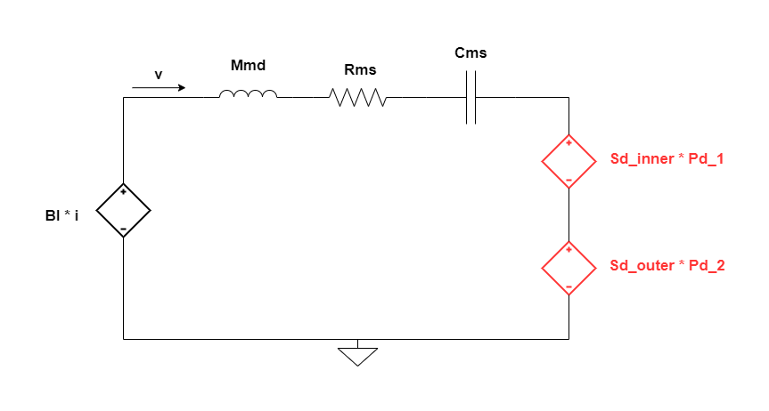
With the expressions derived above for the acoustical lumped model circuit of the driver, the complete circuit transfer function for the whole model is to be derived. These expressions have to be connected back to the mechanical circuit since there is transduction between mechanical and acoustical sections of the driver’s model. Pulling the modified mechanical circuit with dependent sources modelling the acoustical transduction, in here for ease of reference.

The potential differences Pd_1 and Pd_2 shown in the circuit diagram above can be described as
| $Pd\_1 = V_A – V_D$ | (19) |
| $Pd\_2 = V_A – V_B$ | (20) |
The circuit equations developed for the electro-mechanical ONLY circuit of the driver discussed in an earlier post, are to be modified to incorporate the effects of these two new dependent sources. As can be seen, the changes are only to the mechanical circuit while the electrical circuit remains as-is. Reproducing the equations here,
The circuit equation for the electrical circuit is,
$u = R_{e}\cdot i + L_{e} \cdot \dfrac{di}{dt} + Bl \cdot v$ –>(A1)
The modified circuit equation for the mechanical circuit is,
$Bl \cdot i = M_{ms} \cdot \dot{v} + \frac{1}{C_{ms}} \cdot \int{v} + R_{ms} \cdot v \textcolor{red}{+ Pd\_1 \cdot Sd\_inner + Pd\_2 \cdot Sd\_outer}$
$Bl \cdot i = M_{ms} \cdot \dot{v} + \frac{1}{C_{ms}} \cdot \int{v} + R_{ms} \cdot v \textcolor{red}{ + \left (V_A – V_D \right) \cdot Sd\_inner + \left (V_A – V_B \right) \cdot Sd\_outer}$
$Bl \cdot i = M_{ms} \cdot \dot{v} + \frac{1}{C_{ms}} \cdot \int{v} + R_{ms} \cdot v \textcolor{red}{+ V_A \cdot \left (Sd\_inner + Sd\_outer \right)\ -\ V_B \cdot Sd\_outer\ -\ V_D \cdot Sd\_inner } $ –>(B1)
Applying the Laplace transform to (A1)
$\mathscr{L}\{u\} = R_{e} \cdot \mathscr{L} \{i\} + L_{e} \cdot s \cdot \mathscr{L}\{i\} + Bl \cdot \mathscr{L}\{v\}$ –>(A2)
Applying the Laplace transform to (B1)
$Bl \cdot \mathscr{L}\{i\} = M_{ms} \cdot s \cdot \mathscr{L}\{v\} + \frac{1}{s \cdot C_{ms}} \cdot \mathscr{L}\{v\} + R_{ms} \cdot \mathscr{L}\{v\} + V_A’ \cdot \mathscr{L}\{v\} \cdot \left (Sd\_inner + Sd\_outer \right)\ -\ \mathscr{L}\{v\} \left [ V_B’ \cdot Sd\_outer\ +\ V_D’ \cdot Sd\_inner \right ] $ –>(B2)
Isolating $\mathscr{L}\{v\}$ and $\mathscr{L}\{i\}$ terms
$\mathscr{L}\{v\} = \frac{Bl \cdot \mathscr{L}\{i\} }{M_{ms} \cdot s + \frac{1}{s \cdot C_{ms}} + R_{ms} + V_A’ \cdot \left (Sd\_inner + Sd\_outer \right)\ -\ \left [ V_B’ \cdot Sd\_outer\ +\ V_D’ \cdot Sd\_inner \right ]}$ –>(B2a)
Substituting (B2a) in (A2)
$\mathscr{L}\{u\} = R_{e} \cdot \mathscr{L} \{i\} + L_{e} \cdot s \cdot \mathscr{L}\{i\} + Bl \cdot \frac{Bl \cdot \mathscr{L}\{i\} }{M_{ms} \cdot s + \frac{1}{s \cdot C_{ms}} + R_{ms} + V_A’ \cdot \left (Sd\_inner + Sd\_outer \right)\ -\ \left [ V_B’ \cdot Sd\_outer\ +\ V_D’ \cdot Sd\_inner \right ]}$
The Electrical Impedance is then the transfer function computed as
| $G_{ui} = \frac{\mathscr{L}\{u\}}{\mathscr{L}\{i\}}=R_{e} + L_{e} \cdot s + \frac{Bl^2}{M_{ms} \cdot s + \frac{1}{s \cdot C_{ms}} + R_{ms} + V_A’ \cdot \left (Sd\_inner + Sd\_outer \right)\ -\ \left [ V_B’ \cdot Sd\_outer\ +\ V_D’ \cdot Sd\_inner \right ]}$ |
$V_A’$, $V_B’$ and $V_D’$ are expressions with the Laplace transform of Mechanical Velocity $\mathscr{L}\{v\}$ term taken out. Since the rest of the terms in those expressions are constants, the remaining part of the expressions remain the same.
Two sections of the circuit were combined together and clubbed into equivalent impedances before, for ease of analysis. Sharing their expressions below, ( || symbol denotes Parallel Addition)
$Z\_Back = X_{C\_V3}\ ||\ \left [ X_{L\_magVent} + R\_magVent + Z\_rad\_magVent \right ]$ –>(21)
$\begin{align} Z\_Vents &= \left ( Z\_rad\_vent1 + R\_mesh + R\_vent1 + X_{L\_vent1} \right )\ ||\\ &\left ( Z\_rad\_vent2 + R\_mesh + R\_vent2 + X_{L\_vent2} \right )\ ||\\ &…..\\ &…..\\ \\ &\left ( Z\_rad\_vent9 + R\_mesh + R\_vent9 + X_{L\_vent9} \right ) \end{align} $ –>(22)
In the next post, we will look at computing the values for impedances of each of the components discussed here and see what the transfer function equation derived above, gives for those values.