In the last blog post, I said, the DC resistance of the driver as specified by the manufacturer ( $34 \Omega$) could be incorrect and could be a target spec value which they abide by for this product. Electro-acoustics simulation expert, Rene Christensen of Acculution (the same friend I was referring to, in my previous posts) was kind enough to give my blog posts a read and suggested me that the DC resistance might still be $34\Omega$. It could be just that I was only reading the impedance values at high frequencies and the impedance data provided by the manufacturer starts only from 20 Hz. If data were available at lower frequencies, below 20 Hz, it is very much a possibility that the impedance drops further below $36.58 \Omega$. (The plot trend shows that it goes lower beyond 20Hz too, from the looks of it) Since the manufacturer data has the frequency axis plotted on the log-scale, the (super-)low frequency data seems to have been eliminated. (Thank you Rene, for these valuable inputs! 🙂 )
However, for me, the need for finding the minimum impedance value after the first peak was to generate a ‘pseudo’ impedance measurement dataset, for the case when the driver is measured in vacuum. How I plan to achieve that, is by setting the impedance values at high frequencies all to this minimum value thus quashing all the peaks and perturbations beyond the first dominant peak. My reasoning/justification for (still) sticking to the $36.58 \Omega$ value (instead of the manufacturer specified, $34 \Omega$) is that the inductance of the voice coil will impose a higher impedance at higher frequencies, since Inductive Reactance, $X_L = j \cdot \omega \cdot L$. So there is a clear frequency dependency to the impedance contribution by the Voice Coil inductance here, which increases with increasing frequency. (This is my reasoning, for now.. I could very well be proven wrong as I progress on this project. 😀 Nevertheless, it’s all a lesson learned 😉 )
So, now the time has finally arrived to do some Parameter Estimation by curve fitting !!
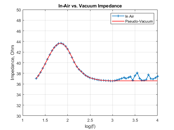
To get you excited a bit, let me reveal the fit right away 😉
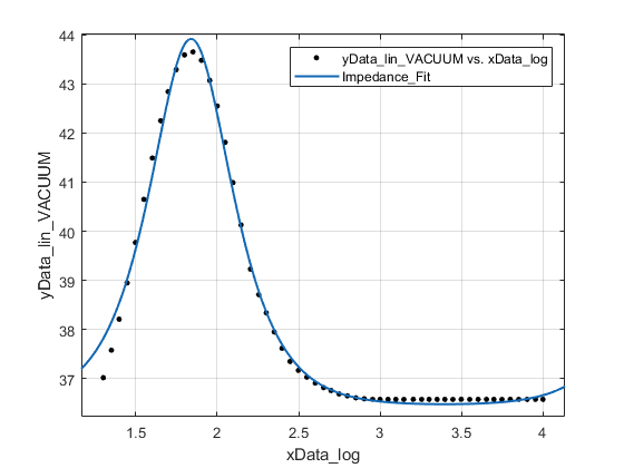
I used the infamous MATLAB Curve Fitting toolbox in this endeavor tonight. (of course, it’s possible to write code to do this task. This toolbox with its GUI is a nice, quick and dirty way to try things out. Maybe, I would have to take the coding route for the later more complicated model which would contain the acoustic section too.)
Here is what the curve fitting toolbox’s UI looks like,
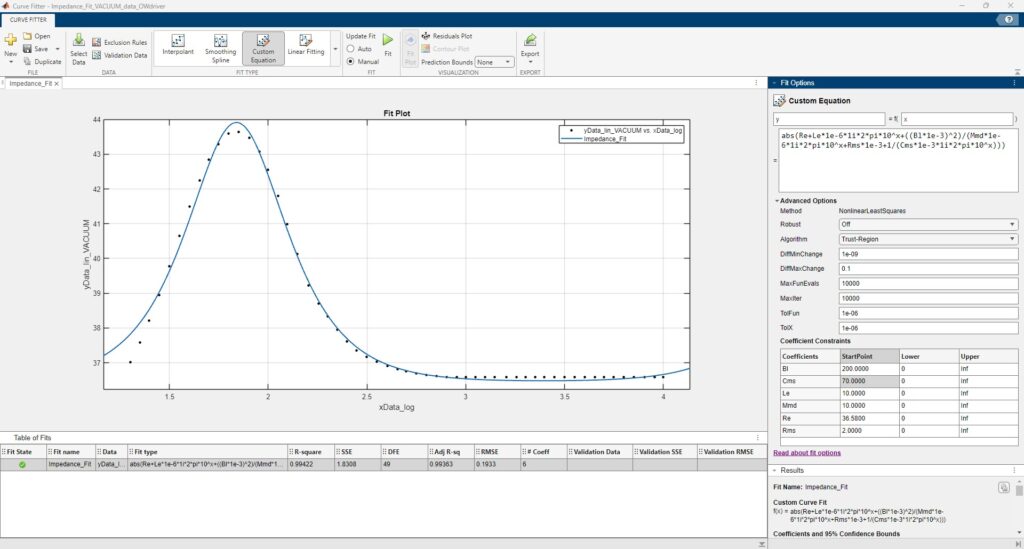
The Nonlinear Least Squares method of fitting was used in the background to achieve this operation. Before getting too excited from seeing a (almost) perfect fit, it’s important to be aware of the fact that, multiple different combinations of parameter values achieve this very same fit. In the 2 hours I spent playing around with the Fitting toolbox, I must have gotten this exact same fit for atleast about 10 to 15 different combinations of the parameter values. By parameters values, I mean, the Bl, Re, Le, Mmd, Rms and Cms values since these are the constituent “control” variables of the impedance equation that we derived in my previous post.
So, an understanding of the magnitude of values for each of the parameters that is expected to be seen for a particular type of driver is very important to have. Another aspect to note is that, the Starting Values (StartPoint column in the right side pane in the above screenshot) chosen before letting the algorithm do the fitting, makes a big difference to how well the fitting algorithm works and also to the quality of results that you get, if you were achieve a “great” fit. So, a word of caution here is that, DO NOT GO BLINDLY BY A GOOD FIT! Check the validity of result values .. ALWAYS!!!
Input expression
As you can see from the screenshot the Curve Fitter expects the expression which is to be fitted to the data. The expression used here is that of the electrical impedance in the Electro-Mechanical (ONLY) model of the driver. As was mentioned in the previous post, this means, it’s what one would see if the driver was measured in VACUUM. (hence, NO Air Load acting on the driver)
abs(Re+Le*1e-6*1i*2*pi*10^x+((Bl*1e-3)^2)/(Mmd*1e-6*1i*2*pi*10^x+Rms*1e-3+1/(Cms*1e-3*1i*2*pi*10^x)))The above expression has a few important aspects to it which are worth discussing,
- The abs(..) of the expression is considered for fitting, since the data provided by the manufacturer is just the magnitude of the Electrical Impedance alone and does not contain the Phase information. However, our expression contains an imaginary term $s= j \cdot \omega$ in it which needs to be eliminated for the fitting algorithm to function. If we had the Phase data available, we could have split the real and imaginary parts of the impedance and used them separately for fitting. But since, we only have the magnitude data available, I’m considering the magnitude of the expression too for fitting.
- The frequency axis datapoints in the provided data are NOT evenly spaced and they are a few orders of magnitude different. As a result, a logarithm of the frequency vector was taken and this array/vector was fed to the Curve Fitter toolbox to form the X-axis. (The Y-axis is however linear since its the linearly spaced impedance data)
- Taking the log of the frequency vector increases the spacing between smaller values and compresses the large values, in effect achieving a linear scale.
- Below are plots of the impedance with a linear and logarithmic frequency axis with the data points marked out by a ‘+’ marker.
- It can be seen how there is a higher number of data points in the lower frequency octaves while the density of points reduces in the higher octaves.
- When the logarithmic axis is used, the data points are evenly spaced out.
- This seems to affect the least squares fitting algorithm (from my past experience atleast) since the weightage of data points changes across octaves and the algorithm tries to over fit in a certain octave which has the highest density of data points while sparsely fitting for the least dense octave.
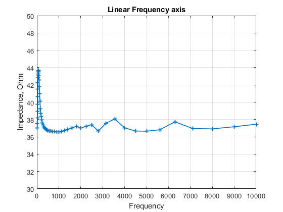
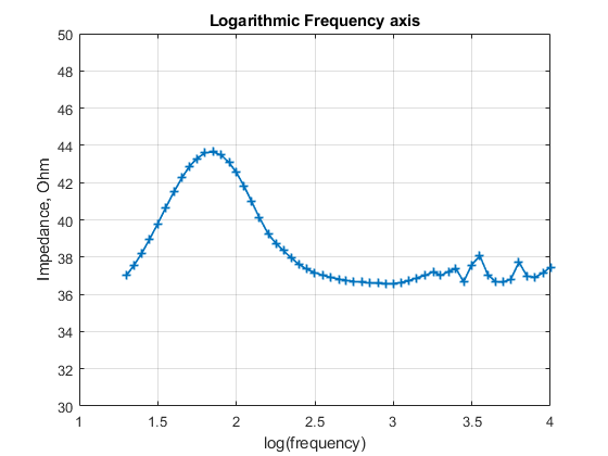
- However, the transformed values after application of logarithm on frequency values should not be used in the calculation of impedance from the expression. Hence the actual frequency value is recomputed in the expression as $10^x$ since the $10^{log10(x)} = x$
- Also if you have not already noticed, the impedance curve used in the fitting toolbox does not have any of the peaks and dips after the first dominant peak. Those have been removed by setting all values to the minimum value ($36.58 \Omega$) from the first occurrence of this value in the impedance data. This way, I am creating a pseudo-vacuum measurement data for this driver to fit the electro-mechanical circuit alone.
- Scaling factors : Each of the parameter is multiplied with a numerical factor in the expression. This is because the toolbox has a limited precision and if the value is too small to fit within that precision, it just displays the value as 0 (zero) which is incorrect. Additionally, the parameters have largely different orders of magnitude by nature. The fitting algorithm also struggles with such variables since the algorithm only looks at them as regular numbers and doesn’t understand the physical significance or the impact of them in the expression provided. So the step sizes are applied by the same magnitude for all variables in each iteration and sometimes fitting fails simply because the correct step sizes were not traversed for some variables which had a vastly different order of magnitude as compared to the rest. So, using scaling factors like here, are a way to bring all parameters to a roughly similar order of magnitude.
Starting Guesses and Bounds
As I mentioned before, starting guesses play an immensely big role in achieving good fit with sensible parameter values. For this some prior knowledge of what to expect for each parameter is necessary or in some cases, alternative measurements could be made to fetch values. For example, the DC resistance could be measured with a simple multimeter and can be used as a starting guess. For the DC inductance of voice coil, perhaps a LCR meter could be. To find the mass of the diaphragm, the diaphragm could be placed on a micro-balance and the actual weight measured. Not all variables can be measured this way though. So, it’s all about finding an optimal balance between practicality and logical reasoning backed judgement for the most part.
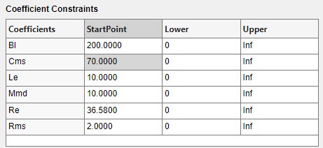
The StartPoint values above are considering the respective scaling factors for each variable, as discussed above. The bounds chosen here are to limit the values to Positive values. More precise bounds could be chosen if you have a better idea of what to expect. Since we estimated the resistance value, $R_{e}$, from the data visually, I have set it to the pre-decided value.
Results
Now the time has arrived to make the final reveal and see what results we get from this fitting operation for each of the parameters.
| Parameter | Units | Scaling Factor | Fitted Value | Actual value=Fitted Value * Scaling Factor |
| Bl | N/A (Newton per Ampere) | 1e-3 | 215.8435 | 215.8435e-3 |
| Cms | m/N | 1e-3 | 524.1332 | 524.1332e-3 |
| Le | H | 1e-6 | 61.9140 | 61.9140e-6 |
| Mmd | kg | 1e-6 | 10.1136 | 10.1136e-6 |
| Re | Ohm | 1 | 36.4635 | 36.4635 |
| Rms | kg/s | 1e-3 | 6.2514 | 6.2514e-3 |
Note: I have represented the moving mass of the diaphragm as Mmd here though in the model I used Mms. Mmd is the correct representation since we are looking at measurements made in Vacuum and hence there is NO air load.
The above values look decent and sensible to me, for this kind of driver. The very low value of the voice coil inductance is expected since it is a very small voice coil with few windings owing to the overall small form factor.
1 Comment