Quite recently, I came across a post on LinkedIn by Ole Wolff, a popular and prominent manufacturer of micro-speaker drivers (among many other products), describing how a Lumped Element model for a micro-speaker could be developed. It was quite brief with only the bare minimum components/attributes of the driver modelled into lumped elements. Perhaps this was done to keep the model simple and compact for the purpose of putting it out in the public domain. I would have liked to see a more detailed ‘acoustic’ section of the model which could (possibly) account for many of the attributes (“kinks”) one could see in the impedance and displacement-Transfer function plots.
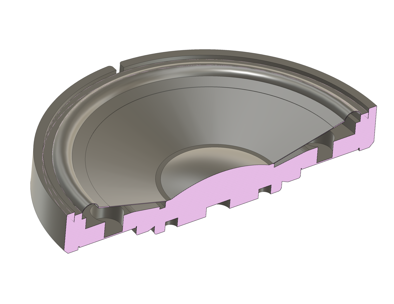
Out of curiosity, I started looking into the catalogue of Ole Wolff micro-speakers on their website. Interestingly Ole Wolff provides a 3D STEP file of their models, though with the limitation of it being merged into a single body and hence hiding some of the details. Additionally on the website, they have impedance and SPL (Sound Pressure Level) plots. The plot data itself i.e., frequency vs. Impedance or SPL data points, is not directly accessible. I might have to manually move my mouse cursor over the plot, point by point and record the data manually. (Perhaps I can get to do that when I’m really fresh and have a ton of patience…;-) ). Since I found these data available on their website, I have an IDEA!! Tada!! I want to try building a model of one of their drivers on my own and see where it gets me. I will document ‘my procedure’ in as much detail as possible with enough math and illustrations in place. I chose the biggest driver on their line-up, the 50mm dia. OWR-5088TA-32 (for no particular reason though.. 😀 ).
Lumped Modelling
I think, I should specify briefly what this method or concept is all about. Though, I don’t see a need to go into the theory of it in too much detail. I can always add ample references to the topic for your perusal.
As the name itself is, this method is about lumping together parts or sections of a device (in this case, a driver) into equivalent electrical circuit elements which exhibit the same behavior as the physical variable (acoustic pressure, velocity, etc.). While doing so, it is important to understand that only those sections of the device can be lumped where a particular physical variable has the same behavior across the dimensions considered. If the physical variable varies drastically within a dimension under consideration, then an equivalent lumped element of that section would be inaccurate in modelling the system behavior. Since we model these physical elements into electrical components (R, L, C, controlled voltage/current sources, etc.), that means, the physical variables like acoustic pressure and velocity are also converted into their electrical equivalents like voltage and current, respectively. (This is true, if an Impedance analogy is deployed. This is what I will be using here to model the driver. There is another analogy called Mobility analogy based on which modelling could be done too. Each analogy has its own pros and cons and suitability benefits for specific domains being modelled.)
Since the physical variable’s magnitude should be the same across a specified dimension being considered for modelling, there is a frequency limit until which any lumped element model is accurate enough. There is no hard limit for this value. However, the frequency corresponding to a wavelength that is at least 10 times the nominal dimension of the section of the device being considered for modelling, would be the limit until which our model is sufficiently accurate. It is important to note that the model does NOT fail abruptly soon after this frequency. The accuracy drops gradually with increasing frequency. We will see what this means as we progress on this project.
Physical elements of interest in the driver
The overall lumped element model of the driver would comprise of the following sections:
- Electrical section : which models the voice coil’s DC resistance and inductance (Note: considers Electrical waves, not acoustic waves)
- Mechanical section : which models the total moving mass of the diaphragm, the damping offered by the mechanical losses in the system and the compliance offered by the suspension (Note: Here, we consider the system’s effect on mechanical waves propagating in the device parts and the frequency limit is considered for mechanical/structural wave propagation and not for the acoustic wave propagation)
- Acoustical section: which models the acoustical behavior of the device and its various components which take part in mechanical-to-acoustical transduction
To model the acoustical section of the driver, there are a few obvious candidates involved like the the effective diaphragm surface (radiation) area (Sd), acoustical compliance offered by the cavity behind the diaphragm, and so on. With micro-speakers whose dimensions are much smaller than conventional, large loudspeaker drivers, every tiny cavity or slit in the system has a considerable impact on the overall driver behavior. All of these aspects, can be used to potentially tune the driver to one’s liking. Or, at the very least, gives us a better picture of why the driver behaves a certain way. Conventional loudspeakers are devoid of such small physical elements in their construction, at least, that they are not small enough to interfere with the driver behavior in the frequency range of interest. Large loudspeakers are also quite open at the back (except for sealed tweeters) unlike micro-speakers.
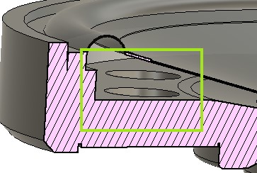
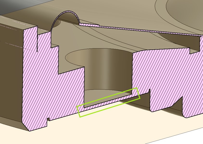
One very interesting example is that, this driver from OW has about 9 venting holes built into the structure behind the diaphragm. These are covered by a tuning paper to add some damping into the venting system so that the pressure behind the diaphragm does not drop rapidly. The tuning mesh covering these holes gives the manufacturer an added degree of control over tuning the whole driver’s performance to his/her liking. Tuning mesh fabrics/papers come in many different specifications of acoustic resistance often specific in MKS Rayls. I will touch upon that, as we get to that point of the modelling. A lumped model which could account for all these attributes would be nice to have to fully understand what’s going on with the driver and also be able to use it for modelling complete built-up systems where one wants to model the driver performance in a coupler or when placed in a cavity, like in a headphone.


In subsequent parts of this blog post, I will go in steps with developing the model of the driver in incremental detail.

1 Comment